How to Run MPC District Toolbox

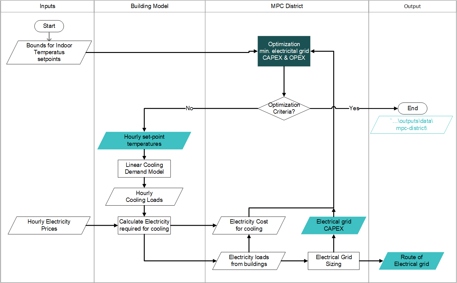
The MPC District Toolbox finds the micro-grid design with the lowest investment and operation costs. The optimization in done in two stages, first, the planning (or design) of the electrical network, and second, the optimization of building temperature setpoints in order to decrease electricity costs. A detailed workflow is shown in the bottom of this page.

The second part is directly calling the MPC Building Toolbox in CEA, please see How to Run MPC Building Toolbox to learn more about MPC Building.

The Optimization Problem

Objective

Minimize annual investment and operation costs of a micro-grid. The investment costs of a micro-grid include: the substations, electricity grid(line), transformers. The operation costs include the maintenance costs of the equiment and electricity costs for cooling in buildings.

Constraints

• Capacity limits corresponding to electric grids, line types.

• Range of the building temperature according to thermal comfort standard.

Variables

• Which buildings are connected to the micro-grid.

• The capacities of substations, electricity grid(line), transformers.

• Hourly temperature set-points for each function in the building

Inputs

1. Range of the building temperature according to thermal comfort standard.

2. Hourly electricity price. The database is located here: ..\CityEnergyAnalyst\cea\databases\Region\systems\electricity_costs.xlsx

Prerequisites

#. Install the license of Gurobi in your computer. you can obtain one in gurobi.com for free for academic purposes. #. Add Gurobi package to the cea environment:

*open anaconda
*do ``conda env update``
*do ``activate cea``
*do ``grbgetkey xxxxxxxxxxxxxxxxxxxxxxxxxxxxxx``
(where xxxxxxxxxxxxxxxxxxxxxxxxxx is the key of your license.)

1. If you are having problems running from pycharm. get today’s version 06.03.2019 or later one. This includes a fix to paths in conda.

Steps

1. Run demand simulation of the case study you wish to optimize.

2. Assign optimization parameters in cea.config:

   [mpc-district]
   time-start = 2005-01-01 00:00:00
   time-end = 2005-01-01 23:30:00
   *set-temperature-goal = constant_temperature, follow_cea, set_setback_temperature
   constant-temperature = 25.0; if the set-temperature-goal = constant_temperature
   *pricing-scheme = constant_prices, dynamic_prices
   constant-price = 255.2; [SGD/MWh]
   *min-max-source = constants, from occupancy, from building.py
   min-constant-temperature = 20.0
   max-constant-temperature = 25.0
   delta-set = 3.0; if min-max-source = from occupancy
   delta-setback = 5.0; if min-max-source = from occupany
   

3. Run ceaoptimizationflexibility_modelmpc_districtplanning_and_operation_optimization.py

4. Check results from optimization in ...scenario\outputs\mpc-district

Outputs

The results from the optimization are saved for each building. In Bxxx_outputs.csv you will find:

• Hourly temperature set-points for each function in the building

• Hourly air flows

• Hourly electricity consumption for cooling

The results of the electricity grid costs and sizes is saved in output_folder.csv

Calculation flowchart

** Please note: To maintain linearity, the cooling demand is calculated by a linearized model instead of the CEA demand module.