What is inside Energy Supply System Optimization in CEA?
CEA provides a optimization tool to complete the analysis of a district. This guide introduce the objectives and variables of the optimization, as well as steps run the tool. This information can help the users to understand the results from the optimization.
Objectives
This tool utilize genetic algorithms to identify energy supply system configurations that minimize the three objectives:
min. Costs: annualized capital costs and operational costs
min. Emissions: annual green house gas emissions from the technology operation
min. Primary Energy: annual primary energy consumptions
The results from the optimization is a collection of pareto-optimum solutions.
Optimization Variables
Beside the objectives, the main outputs from the optimization is the energy supply system configurations. Each pareto-optimum solution implies a unique energy supply system configuration. A configuration is combination of energy supply technologies and sizes. All possible configurations that is incorporated in the CEA is presented in this figure:
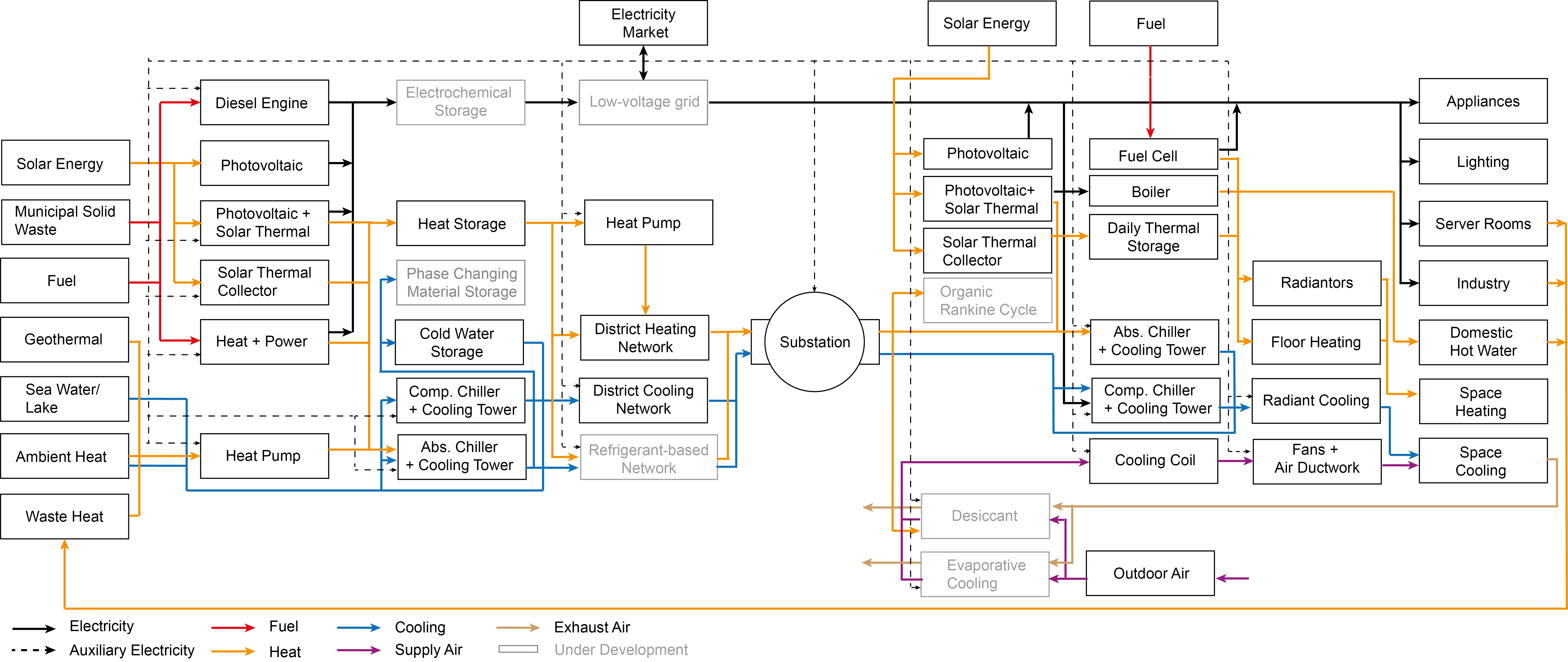
Supply technology selection and sizing
Each perato-optimum solution includes a set of technologies that are installed, and the respective capacities. The district scale technologies are connected to micro-grids or thermal networks to supply the energy to individual buildings in a district.
Thermal network design
Each perato-optimum solution also specify how many buildings are connected to a district heating or cooling network. The main trade-off is between the capital expenditures on constructing the pipes and energy savings from using centralized plants or utilizing on-site renewable energy potentials. The buildings that are not connected to the thermal networks are supplied by decentralized technologies installed at buildings.
Steps to Run The Tool
Do Step 1, 2, 3, 5, 9 in How to do analyses with CEA?
Assign optimization parameters <#Optimization-Parameters>.
Run decentralized_building_main.py or the equivalent toolbox
Run optimization_main.py or the equivalent toolbox
Run multicriteria > main.py or the equivalent toolbox
Check results from optimization in
...outputs/data/optimization/network/all_individuals.csvor using the plotting tools for optimization (Step 10 in How to do analyses with CEA?)
Optimization Parameters
For this optimization, the users can adjust four optimization parameters or use the default numbers.
district-heating-network: Boolean, describes if a district heating system should be optimized. Default is true
district-cooling-network: Boolean, describes if a district cooling system should be optimized. Default is false
detailed-electricity-pricing: Boolean, describes if a district cooling system should be optimized. Default is false
population-size: Boolean, describes if a district cooling system should be optimized. Leave this field empty to use the standard 92 by Deb et al.,2014.
number-of-generations: number of iterations of GA algorithm (NSGA-III by Dep et al., 2014). Default is 100
random-seed: Random seed to make it easy to replicate the results of the scenarios. Default 100
crossover-prob: Probability of crossover. Default 0.9
mutate-prob: Probability of mutation. Default 0.1
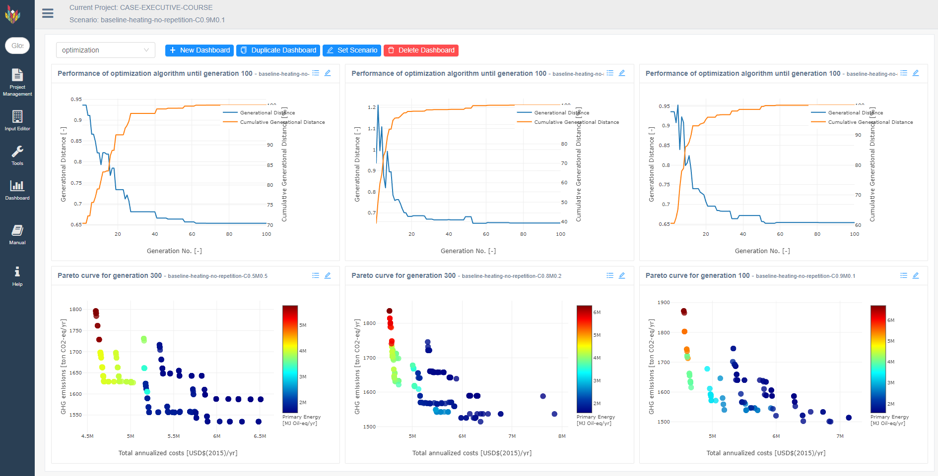
These parameters are case-study dependent and need to be tuned based on the user requirement. The default values provided are to act like a beacon in the research. The next figure presents a comparison of three combinations of crossover-prob and mutate-prob. The first row presents the Generational distance for every generation for each of the three cases. The second row presents the pareto curves for each curve.
NOTE: As Genetic Algorithm, which is stochastic in nature, is being used as an optimization algorithm, the results might not always be exact. So if there are 5 runs of the optimization, there is no guarantee that all 5 runs will yield the same solution, but the solutions will be in close proximity. For example, if in a minimization problem, the result in first run is 30056712, the second run might be 30045891 and the third run might be 30050025. But if the results are normalized they are within 0.1% of the each other. An ideal way to run Genetic Algorithm is to do multiple runs and take the best out of it and also note the worst result you might get from the optimization.
More on what’s behind the scene
Want to know how to understand the result files?
There are tremendous amount of information that is generated through the optimization process. Your go-to file to start with is case studyoptimizationslaveAll_individuals.csv. This files includes objectives and variables of all individuals evaluated by the optimization. To navigate through the rest of the files in the case studyoptimization folder, please refer to Files generated by the CEA.
Want to know more about the master and slave structure?
This optimization follows a bi-level structure. In the master level, the configurations are determined, and the slave level, the hourly operation is determined. To dig more into the structure of this optimization, please refer to these workflow diagrams.