How are schedules defined?

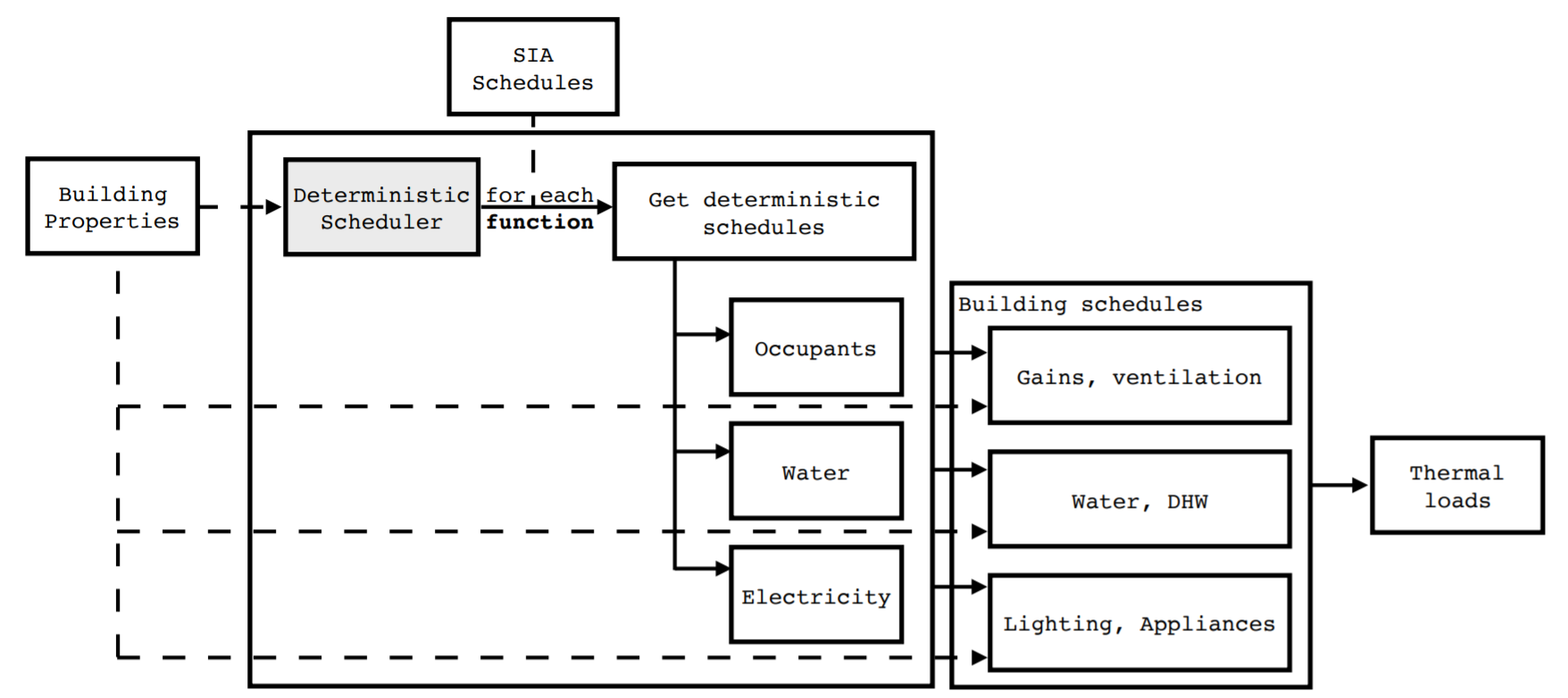
Deterministic

CEA includes deterministic schedules for 18 building functions (such as residential, office, school…) derived from SIA standard 2024 [1]. Schedules stored in occupancy_schedules.xlsx are generally separated into decimal probabilities for the following, with i denoting the building function:

P _occupancy,i : hourly probability of occupancy
P _{lighting/appliances,i} : hourly probability of lighting and appliance use
P _dhw,i : hourly probability of domestic hot water (DHW) use
P _monthly,i : monthly probability of building function use
Occ _i : occupancy density in (m ² / person)

Other variables used to calculate the loads include:

Share _i : percentage of the building’s net floor area that corresponds to the function, i
NFA is the building’s net floor area
e _lighting,i : energy demand of lighting per square meter (W / m ²)
e _appliances,i : energy demand of appliances per square meter (W / m ²)
d _dhw,i : daily demand for hot water (litres/person/day)

At the beginning of the simulation for each building, yearly schedules of occupant presence (N _people) and associated indoor comfort parameters, as well as schedules of electricity (E _light and E _appliances) and hot water consumption (V _dhw) are calculated as a simple average:

\[ \begin{align}\begin{aligned}N_{people}(t)= \sum_i{P_{occupancy,i}(t)\cdot{P_{monlthy,i}(t)\cdot{Occ_i}\cdot{Share_i}\cdot{NFA}}}\\E_{lighting}(t)= \sum_i{P_{lighting/appliances,i}(t)\cdot{P_{monlthy,i}(t)\cdot{e_{lighting,i}}\cdot{Share_i}\cdot{NFA}}}\\E_{appliances}(t)= \sum_i{P_{lighting/appliances,i}(t)\cdot{P_{monlthy,i}(t)\cdot{e_{appliances,i}}\cdot{Share_i}\cdot{NFA}}}\\V_{dhw}(t)= \sum_i{P_{dhw,i}(t)\cdot{P_{monlthy,i}\cdot{d_{dhw,i}}(t)\cdot{Occ_i}\cdot{Share_i}\cdot{NFA}}}\end{aligned}\end{align} \]

These schedules are then passed on to the thermal loads module of CEA, where they represent either demands to be satisfied for the building in question or internal gains that need to be accounted for in the thermal model.

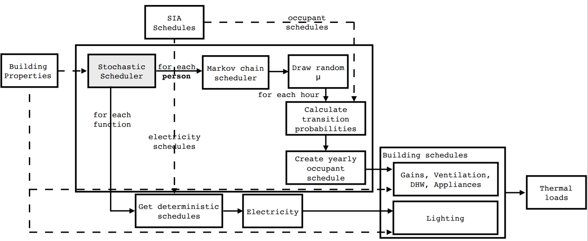
Stochastic

In addition to this deterministic model, CEA includes the option of using the occupant presence model of Page et al [2]. as an alternative occupant modeling option in the tool. In this model, each occupant’s presence is modeled as a two-state Markov process. Transition probabilities between the states “absence” (state 0) and “presence” (state 1) are defined at each hour of the year for each user in the area. For an occupant in a space with function i, the probability of an occupant being in the space in question P _i (t) is taken from the deterministic schedule discussed above as follows:

\[P_i(t)=P_{occupancy,i}(t)\cdot{P_{monlthy,i}(t)}\]

At each time step, the transition probabilities between these states are calculated as follows:

\[ \begin{align}\begin{aligned}T_{11}(t) =\frac{P(t)-1}{P(t)}\cdot{T_{01}(t)}+\frac{P(t+1)}{P(t)}\\T_{01}(t) =\frac{\mu-1}{\mu+1}\cdot{P(t)}+P(t+1)\end{aligned}\end{align} \]

Where T ₁₁ (t) is the probability of the occupant staying in the room at time t+1 given that the occupant was present at time t and T ₀₁ (t) is the probability of the occupant arriving at time t+1 given that they were not present at the previous time step.

μ is a so-called “parameter of mobility,” assumed by the authors to be constant for simplicity:

\[ \begin{align}\begin{aligned}\mu = \frac{T_{01}(t)+T_{10}(t)}{T_{00}(t)+T_{11}(t)}\\where:\\T_{00}(t) + T_{01}(t) = 1\\and\\T_{10}(t) + T_{11}(t) = 1\end{aligned}\end{align} \]

The only parameter that needs to be estimated is μ.